
Table of Contents
Linking attacks in genomic studies
Several studies have shown that releasing gene expression data can leak private information about individuals (Harmanci & Gerstein 2016; Walker et al. 2024).
This is how an adversary would do it:
-
A study releases anonymized expression data with sensitive disease labels (e.g., HIV status)
-
Gain access to eQTL summary statistics by examining how genotypes correlate with expression
-
Predict genotypes from expression vectors by quantizing eQTL-predictable values to match possible 0 (homozygous reference), 1 (heterozygous), 2 (homozygous alternative) alleles.
-
Match the predicted genotypes (bins) to a reference genotype database
-
A successful match over many SNPs will probabilistically identify a targeted individual
Walker et al. showed 93%+ linking accuracy on single-cell data, even with all the inherent interference.
Can we release a bit noisy yet safer eQTL summary statistics?
One way to mitigate this is to release differentially private eQTL summary statistics instead of exact ones. Can we add enough noise to prevent linking while keeping the statistics useful?
Let's build a toy example:
- $n = 100$ individuals
- One SNP with minor allele frequency 0.3
- Gene expression as a function of genotype: $E = \beta \cdot G + \epsilon$ (an eQTL)
library(ggplot2)
set.seed(42)
n <- 100
maf <- 0.3

## genotype (private) and expression (released in the study)
G <- rbinom(n, size = 2, prob = maf)
E <- 0.5 * G + rnorm(n)

dat <- data.frame(id = 1:n, genotype = G, expression = round(E, 3))
head(dat)
##   id genotype expression
## 1  1        2      1.322
## 2  2        2      0.216
## 3  3        0      1.576
## 4  4        1      1.143
## 5  5        1      0.590
## 6  6        1      0.777
The study releases the expression data (anonymized) along with disease labels. The genotypes are private. But the eQTL summary statistic, i.e., the regression coefficient $\hat{\beta}$ from $E \sim G$, captures the genotype-expression relationship:
beta_hat <- coef(lm(E ~ G))
cat("eQTL intercept:", beta_hat[1], "\n")
## eQTL intercept: -0.1238356
cat("eQTL effect: ", beta_hat[2], "\n")
## eQTL effect: 0.6449423
An attacker with access to these exact eQTL statistics can predict genotypes from expression. Each eQTL is a separate marginal regression, one SNP and one gene:
$$ E_k = \beta_k G_k + \epsilon_k, \quad k = 1, \ldots, p $$
With many such pairs, the attacker builds a genotype profile for each individual: for each gene $k$, predict the most likely genotype $G_k$ given the observed expression $E_k$ and the released $\hat{\beta}_k$. More eQTLs = more bits of genotype information = more accurate linking.
## p independent eQTLs, each a marginal regression
p <- 20
G_multi <- matrix(rbinom(n * p, size = 2, prob = maf), nrow = n, ncol = p)
E_multi <- matrix(nrow = n, ncol = p)
beta_true_vec <- rep(0.5, p)

for (k in 1:p) {
  E_multi[, k] <- beta_true_vec[k] * G_multi[, k] + rnorm(n)
}

## attacker runs marginal regression per eQTL
betahats <- sapply(1:p, function(k) coef(lm(E_multi[, k] ~ G_multi[, k]))[2])

## predict genotype per eQTL: round(E / beta) clipped to {0, 1, 2}
G_predicted <- sapply(1:p, function(k) {
  pmin(pmax(round(E_multi[, k] / betahats[k]), 0), 2)
})

## how many genotypes does the attacker get right?
accuracy <- mean(apply(G_predicted == G_multi, 2, mean))
cat("Genotype prediction accuracy:", round(accuracy, 3), "\n")
## Genotype prediction accuracy: 0.425
## linking: match each individual's predicted genotype profile to the reference
## using Hamming distance
link_correct <- 0
for (i in 1:n) {
  dists <- apply(G_multi, 1, function(g_ref) sum(g_ref != G_predicted[i, ]))
  link_correct <- link_correct + (which.min(dists) == i)
}
cat("Linking accuracy:", link_correct, "/", n, "\n")
## Linking accuracy: 3 / 100
Each eQTL gives a noisy estimate of one SNP's genotype. But combined across many eQTLs, the predicted genotype profile becomes unique enough to link individuals to a reference database. This exactly how we do identity attack.
Protecting eQTL statistics with differential privacy
Before releasing $\hat{\beta}$, we can add random noise while calibrating the vulnerability of the data release. For a simple linear regression, changing one person's record shifts $\hat{\beta}$ by at most some $\Delta$.
A common option is to add random jitter sampled from a Laplace distribution, as used for the sparse coding, L1-penalty, or LASSO. Namely, we achieve $\epsilon$-DP by adding noise sampled from $\mathsf{Laplace}(0,\Delta/\epsilon)$
set.seed(42)
## sensitivity: how much can one person change a marginal beta?
## for bounded expression in [-B, B]:
B <- 3

## Laplace noise generator
rlaplace <- function(n, scale) {
  u <- runif(n, -0.5, 0.5)
  -scale * sign(u) * log(1 - 2 * abs(u))
}

## conservative sensitivity for a marginal regression coefficient
sensitivity <- 2 * B / n

## compare linking accuracy under different epsilon values
epsilons <- c(0.1, 0.5, 1.0, 10)

par(mfrow = c(2, 2))
for (eps in epsilons) {
  ## add Laplace noise to each marginal beta
  beta_noisy <- betahats + rlaplace(p, scale = sensitivity / eps)

  ## attacker predicts genotypes using noisy betas
  G_pred_noisy <- sapply(1:p, function(k) {
    pmin(pmax(round(E_multi[, k] / beta_noisy[k]), 0), 2)
  })

  ## linking via Hamming distance
  linked <- 0
  for (i in 1:n) {
    dists <- apply(G_multi, 1, function(g) sum(g != G_pred_noisy[i, ]))
    linked <- linked + (which.min(dists) == i)
  }

  acc <- mean(G_pred_noisy == G_multi)
  plot(1:p, betahats, pch = 19, col = "black", ylim = range(beta_noisy, betahats),
       xlab = "eQTL index", ylab = "Effect size",
       main = bquote(epsilon == .(eps) ~ " (linked " ~ .(linked) ~ "/" ~ .(n) ~ ")"))
  points(1:p, beta_noisy, pch = 4, col = "red")
  legend("topright", legend = c("true", "noisy"), pch = c(19, 4), col = c("black", "red"), cex = 0.8)
}
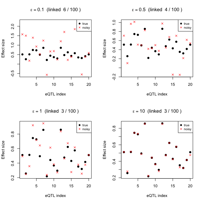
- At $\epsilon = 0.1$ (strong privacy), the attacker's predictions are essentially random. But the coefficients deviate too much from the true one.
- At $\epsilon = 10$ (weak privacy), the predictions are nearly as good as the exact case. But the data security breach may occur.
- The researcher must choose $\epsilon$ based on the acceptable trade-off between utility and privacy
The cost: can we still detect true eQTLs?
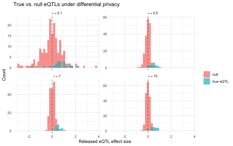
Privacy is only useful if the released statistics are still scientifically meaningful. Let's simulate a more realistic scenario: many genes, some with real eQTLs and some without, and ask whether we can still distinguish them after adding DP noise.
set.seed(123)
n_genes <- 200
n_causal <- 20  # true eQTLs

## one SNP, same genotype vector for simplicity
G_util <- rbinom(n, size = 2, prob = maf)

## simulate expression for each gene
beta_sim <- rep(0, n_genes)
beta_sim[1:n_causal] <- rnorm(n_causal, mean = 0.5, sd = 0.2)

E_mat <- sapply(beta_sim, function(b) b * G_util + rnorm(n))

## compute true eQTL betas
beta_est <- apply(E_mat, 2, function(e) coef(lm(e ~ G_util))[2])

## add DP noise at different epsilon levels
epsilons <- c(0.1, 0.5, 1.0, 10)

results <- do.call(rbind, lapply(epsilons, function(eps) {
  if (is.finite(eps)) {
    noisy <- beta_est + rlaplace(n_genes, scale = sensitivity / eps)
  } else {
    noisy <- beta_est
  }
  data.frame(
    gene = 1:n_genes,
    beta_noisy = noisy,
    causal = ifelse(1:n_genes <= n_causal, "true eQTL", "null"),
    epsilon = if (is.finite(eps)) paste0("epsilon == ", eps) else "epsilon == Inf"
  )
}))

ggplot(results, aes(x = beta_noisy, fill = causal)) +
  geom_histogram(bins = 40, alpha = 0.7, position = "identity") +
  facet_wrap(~epsilon, scales = "free_y", labeller = label_parsed) +
  geom_vline(xintercept = 0, linetype = "dashed", color = "grey40") +
  labs(x = "Released eQTL effect size", y = "Count",
       title = "True vs. null eQTLs under differential privacy",
       fill = "") +
  theme_minimal()
What $\epsilon$ actually promises: It's all about membership attack/protection
So what's the theory behind it? We don't want to reveal whether an individual's data point is included by adding some noise with an $\epsilon$-DP guarantee.
$$\Pr{\text{stat with Laplace noise} \mid \text{you're in DB}} \le e^{\epsilon} \times \Pr{\text{stat with Laplace noise} \mid \text{you're out of DB}}$$
The intuition is that an attacker who sees the output can't tell whether your data point is in or out since the output would have looked essentially the same regardless.
- Small $\epsilon$ (say 0.1): the two versions are nearly indistinguishable, so your privacy is strong, but we had to add a lot of noise, so the statistics are less accurate.
- Large $\epsilon$ (say 10): little noise, accurate statistics, but now your presence visibly shifts the output, so privacy is weak.
We can make this concrete. Suppose before seeing the data the attacker gives some odds that you're in the study. After seeing the released statistics, they update those odds. The $\epsilon$-DP guarantee says this update can only be so large: the odds can grow (or shrink) by at most a factor of $e^{\epsilon}$:
$$\frac{\text{odds you're in, after seeing the output}}{\text{odds you're in, before}} \le e^{\epsilon}$$
So $\epsilon$ has a direct reading as a worst-case multiplier on the attacker's betting odds:
| $\epsilon$ | $e^{\epsilon}$ | plain reading |
|---|---|---|
| 0.1 | ≈ 1.1 | odds of guessing membership rise by at most ~10% |
| 0.5 | ≈ 1.6 | at most ~1.6×, namely a 50/50 attacker reaches at most ~62% |
| 1.0 | ≈ 2.7 | at most ~2.7×, namely a 50/50 attacker reaches at most ~73% |
Here is a concrete example. Say the attacker starts at even odds, a coin flip, 50/50 on whether you're in the study. With the exact statistic released, suppose the evidence is strong enough to push their odds up by 100 fold, to 100-to-1. That's a jump from 50% to about 99% confidence that you're in, essentially identified.
Now suppose we release the statistic under $\epsilon$-DP instead. The odds can move by at most $e^{\epsilon}$, so:
- At $\epsilon = 1$: the 100 fold increase of the security breach is capped at $e^1 \approx 2.7\times$, i.e. odds of at most 2.7-to-1, or about 73% confidence, still uncertain.
u- At $\epsilon = 0.5$: capped at $e^{0.5} \approx 1.6\times$, odds of at most 1.6-to-1, or about 62% confidence, only a nudge above the coin flip.
- At $\epsilon = 0.1$: capped at $e^{0.1} \approx 1.1\times$, odds of at most 1.1-to-1, or about 52%, barely better than the coin flip they started with.
The protocol isn't really making the attack impossible. Instead, we make its guesswork much less likely.