Causal Inference in Genomics
TL;DR. We reinvent traditional bioinformatics methods to ascertain the causality of discoveries made in high-dimensional omics data.
Massive data generation in genomics has transformed the methodology and practice of researches in medicine and human biology. A common practice of research is genomic and functional genomic profiling of hundreds of individuals. If desired data is not available, large consortium-level projects and collaborations can often meet the needs. In terms of both volume and dimensionality, the sizes of genomics data have exploded in the past decade, and it is not hard to predict that the speed of data accumulation will be further accelerated.
Genomics has made a breakthrough in medicine and science, armed with two powerful scientific methods–hypothesis testing and machine learning (ML). Hypothesis testing with well-designed null distributions proves meaningful scientific discoveries are made on the observed data. Likewise, a traditional ML method is designed to efficiently search the most plausible models from a particular class of models, mainly focusing on minimizing generalization errors on the observed data. However, biology’s ultimate question is perhaps more about unobserved principles, asking counterfactual “what if” questions, rather than simply describing phenomena. We desire to uncover causal mechanisms and laws underlying observations and ultimately provide testable cause-effect relationships.
Causal inference based on a causal structure model
Most causal inference concepts based on a structural equation model are already adopted in a carefully designed biological experiment. We can trace back to Sewall Wright’s path diagram model. For instance, an experimental proof demonstrating the effect of a gene “X” to some trait “Y” would require two types of interventions that disruption of the gene X makes changes to the trait Y, and recovery of the gene can attenuate the disrupted functions. However, a common practice of high-throughput data analysis often lack such intervention steps, but hurriedly arrive at some conclusion based on observed correlation patterns. Many of these correlations may turn out non-causal but somewhat confounded by unobserved variables.
Identification of causal effects by an instrumental variable (mediation)
The key concept is an intervention. However, introducing an intervention is often impossible for technical and ethical reasons, and there are so many things to perturb to test the effects. Moreover, the effects of causal mechanisms might be too small to quantify within a reasonable statistical error reliably. How do we ascertain causal effects by intervention?
Stepping back, let us think about two principal axes of the data generation process: the breadth of population-level measurements across tens of thousands of samples and the depth of regulatory genomics across multiple layers of causal mechanisms, seeking a precise answer up to a single-cell resolution.
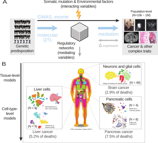
We can recognize a causal direction from genetic information to phenotypic variation if we consider that genotypes are shaped by nature’s randomized controlled trial (RCT), or natural interventions. Given that, the goal is to identify causal mediators located in the middle of the above causal diagram. In the context of genome-wide association studies (GWAS), the mediator variables include relevant cell types and target genes derived from tissue-level or cell-type-level eQTL data.
Removing unwanted variability by “control” data
Many scientific discoveries are best represented as a set of contrastive statements, such as “A rather than B” ( Peter Lipton) because such a contrastive explanation clarifies our claim’s scope and basis. The validity of causal argument can be empirically justified by triangulation of contrastive arguments (Lipton 1991). Therefore, an essential aspect of our research should focus on finding a suitable set of null hypotheses (non-causal facts) to be contrasted against our theory of interest to uphold. What are non-causal effects that may obfuscate the activity of scientific research? Are they generated uniformly at random? In practice, it is hard to characterize non-causal effects without considering confounding variables, and confounders create unwanted non-zero correlations between cause and effect variables.
Confounder correction is a causal inference problem. So, we need to ask the question of identifiability, such as, “How do we know this variable is a confounder?” or “What is a legitimate criterion that distinguishes between causal and non-causal effects?”. We could start our journey by asking:
-
Are there any control data on which we can safely claim that there is no causal effect whatsoever?
-
Are they already available/observed? Or, should we construct/estimate them?
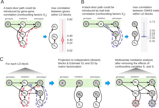
Like many research problems, control data (or variables) are hidden, yet to be estimated. In the mediation problem, for instance, we need to think about how to characterize confounding variables that relate two mediators (genes, M1 and M0) (A) and the other type of confounders between different phenotypes (B). Unless we adjust these confounding effects, mediation effects are not identifiable by statistical inference. Fortunately, we can construct control data that only include non-genetic correlation structures by exploiting human genetics’s nature. Since genetic correlations are confined within each linkage disequilibrium (LD) block, we can defuse putative causal effects by projecting summary statistics onto a different, independent LD block (C). We actively construct control data to identify confounding variables.
On this matter, we are broadly interested in general genomics problems, not just statistical genetics ones. Although the definition of a confounding variable is problem-specific, we seek to design probabilistic models and ML algorithms that semi-automate the overall process. The methods will indicate a set of putative confounding variables with a level of uncertainty by taking input data and prior knowledge (e.g., known causal and non-causal variables).
A potential outcome framework for causally-differential expression analysis
Recently, our interest in Donald Rubin’s potential outcome framework grew, and started thinking about a type of causal problems that can be better approached by Rudin’s causal model (RCM).
“Bayesian” causal inference for single-cell data analysis
As a first step, we revisit commonly-practised bioinformatics problems and reformulate them in RCMs. The ultimate goal of RCM is to ask and estimate counterfactual questions. Causality is tied to an action (doing), rather than an observation (seeing), and counterfactual causal inference seeks to take an impossible action and estimate its effects.
Suppose we want to test the causal statement: A gene expression of Y was changed because of a disease X, i.e., $X \to Y$ with a directed edge (going beyond $Y \sim X$). We define $X$ to take 1 or 0 for “yes” or “no” and the resulting gene expression $Y$ to take a real number. In observational studies, including most high-througput assays, we observe a pair of $X_{i}$ and $Y_{i}$ for an individual $i$; there, the observed $Y_{i}$ value stems from the observed $X_{i}$, either 1 or 0, not both. E.g.,
| $i$ | X | Y(0) | Y(1) |
|---|---|---|---|
| 1 | 0 | $Y_1$ | ? |
| 2 | 1 | ? | $Y_2$ |
| 3 | 1 | ? | $Y_3$ |
| 4 | 0 | $Y_4$ | ? |
| $\vdots$ |
In counterfactual inference, we want to infer the other unobserved and not observable cases. For $X_{i}=1$, we want to know the potential outcome of $Y_{i}$ if we had $X_{i} = 0$, and vice versa. RCMs generally translate the underlying problem as a Bayesian imputation problem, or a matrix completion problem, which contains at least 50% of missing values. Provided an accurate Bayesian imputation method, we can quantify individual-level causal effects, $Y_{i}(1) - Y_{i}(0)$, as well as average causal effects, $\mathbb{E}\left[Y(1) - Y(0)\right]$. This is truly substantial advancement because we no longer worry about identifiability but focus on a statistical inference problem.
Well, there is a catch. In traditional omics data analysis, such an imputation problem is pretty challenging unless we have a good understanding of the data-generating process, which is often a black box to us. For one individual, we only have one data point $Y_{i}$ unless we borrow information from related genes. We might have to rely on faithful pretreatment variables $W$ as in a causal path, $W \to X \to Y$, and construct propensity scores to reweight observed samples.
However, single-cell data provide a unique opportunity for modelling high-dimensional omics profiles. A clear advantage over bulk data is simply that we have more data points per sample (individual). Assuming that single-cell profiling’s sensitivity will become better each year, it is not too far until we can achieve reliable and accurate Bayesian imputation methods–not only the observed values but also the counterfactual values.