Table of Contents
TL;DR: Consider transparent parameterization for a partially identified model if a strong dependency with prior distributions was found in Bayesian causal inference.
Set-up:
- $Z \in {0,1}$: a randomized assignment or "instrument"; $Z$ is a treatment, presumed to be randomized, e.g., the assigned treatment.
- $X \in {0,1}$: an exposure measure; $X$ is an exposure subsequent to treatment assignment.
- $Y \in {0,1}$: a final response; $Y$ is the response.
- There might be confounding on $X$ and $Y$
Goal: What is the effect of $X$ on $Y$?
Identifiability matters, so we should make which parts are identifiable and which parts not.
It is often argued that identifiability is of secondary importance in a Bayesian analysis provided that the prior and likelihood lead to a proper joint posterior for all the parameters in the model. [...] we argue that partially identified models should be re-parameterized so that the complete parameter vector may be divided into point-identified and entirely non-identified subvectors. Such an approach facilitates "transparency", allowing a reader to see clearly which parts of the analysis have been informed by the data
A potential outcome problem
We further define:
- $X^{(z=0)}$ or $X^{(z=1)}$ for the treatment a patient would receive if assigned to $Z=z$
- $Y^{(x,z)}$ for the outcome for a given patient if they were to be assigned to $Z = z$, and then were exposed to $X = x$.
Why is it a potential outcome problem? A person may or may not take a pill (exposure) in relations with the assignment $Z$:
| compliance type | $X^{(z=0)}$ | $X^{(z=1)}$ |
|---|---|---|
| Never Taker (NT) | 0 | 0 |
| Complier (CO) | 0 | 1 |
| Defier (DE) | 1 | 0 |
| Always Taker (AT) | 1 | 1 |
What are the potential responses regarding the exposure and response variables?
| response type | $Y^{(x=0)}$ | $Y^{(x=1)}$ |
|---|---|---|
| Never Recover (NR) | 0 | 0 |
| Helped (HE) | 0 | 1 |
| Hurt (HU) | 1 | 0 |
| Always Recover (AR) | 1 | 1 |
Pearl (2000) considering a subset of data
If we only consider "possible" (or partially factual) cases, $Z=0$ implies $X=0$, which leaves us only NT and CO. We can assume $Z \to X \to Y$ but no direct path $Z \to Y$ that skips over $X$.
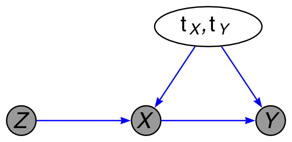
$$\textsf{ACE}(X \to Y) \equiv \mathbb{E}\left[Y^{(x=1,z)} - Y^{(x=0,z)}\right]$$
Pearl proposes analyzing the model by placing a prior distribution over $p(tX , tY)$ and then using Gibbs sampling to sample from the resulting posterior distribution for ACE($X \to Y$).
Sensitivity to the choice of prior distribution over compliance and response types:
If the model were identified, we would expect such a change in the prior to have little effect (the smallest observed count is 12). However, as the plot shows, this perturbation makes a considerable difference to the posterior.
$$\textsf{ACE}(X \to Y) = \pi_{\textsf{CO}}\left(\gamma_{\textsf{CO}}^{(1,\cdot)} - \gamma_{\textsf{CO}}^{(0,\cdot)}\right) + \pi_{\textsf{NT}}\left(\gamma_{\textsf{NT}}^{(1,\cdot)} - \gamma_{\textsf{NT}}^{(0,\cdot)}\right)$$
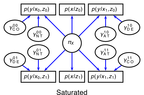
Why is it not fully identified? The following factor graph (or PGM-like) well summarizes.

We need to calculate two types of differences:
- $\gamma_{\textsf{CO}}^{(1,\cdot)}$ vs. $\gamma_{\textsf{CO}}^{(1,\cdot)}$
- $\gamma_{\textsf{NT}}^{(1,\cdot)}$ vs. $\gamma_{\textsf{NT}}^{(1,\cdot)}$
Here, $\gamma_{\textsf{NT}}^{(1,\cdot)}$ has to rely on Bayesian sampling over some prior distribution. Okay, we could average out unidentified random variables, but if they were not attached to any part of the data, we would resort to the shape of the prior distribution.
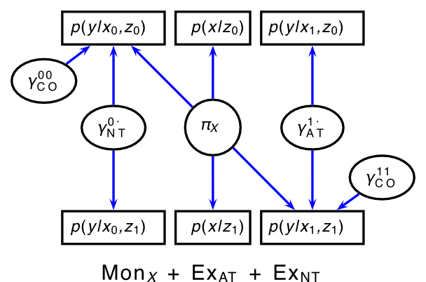
From a saturated model to the model considered by Hirano et al. (2000)
We need to consider more data to be able to identify all the parameters:
Or at least, we should make each parameter attached to measurable sufficient statistics with a bit more assumptions:
-
Monotonicity of $X$ of $Z$: There are no defiers, meaning $X^{(0)} \le X^{(1)}$.
-
Stochastic exclusion of NT: $\gamma_{NT}^{(0,1)} = \gamma_{NT}^{(0,0)}$
-
Stochastic exclusion of AT: $\gamma_{AT}^{(1,1)} = \gamma_{AT}^{(1,0)}$
Intent-to-treat effect (Hirano et al. 2000):
$$\textsf{ITT}(\textsf{compliance type}) = \mathbb{E}\left[ Y^{(X(1),1)} - Y^{(X(0),0)} | \textsf{compliance type}\right].$$
We can parameterize this by:
-
$\textsf{ITT}(\textsf{CO}) = \gamma_{CO}^{(x=1,z=1)} - \gamma_{CO}^{(x=0,z=0)}$
-
$\textsf{ITT}(\textsf{NT}) = \gamma_{NT}^{(x=0,z=1)} - \gamma_{NT}^{(x=0,z=0)} = 0$ (by the above exclusion assumption 2)
-
$\textsf{ITT}(\textsf{AT}) = \gamma_{AT}^{(x=1,z=1)} - \gamma_{AT}^{(x=1,z=0)} = 0$ (by the above exclusion assumption 3)
My takeaway
-
I didn't go over all the inequalities laid out by the authors, so there is more clarity to be found.
-
Working out some sort of factor graph representation will be useful to see which parameters are identifiable.
-
I wonder if we can design an algorithm that detects partially or fully identified model parameters.
-
A Bayesian inference engine geared toward "integrate out" will not always yield identifiable results.