Table of Contents

Generative models

Discrete (non-mixed) stochastic block models

One of the most well-known examples in early social network study is this: An Information Flow Model for Conflict and Fission in Small Groups Zachary (1977).

At the beginning of the study there was an incipient conflict between the club president, John A., and Mr. Hi over the price of karate lessons. Mr. Hi, who wished to raise prices, claimed the authority to set his own lesson fees, since he was the instructor. John A., who wished to stabilize prices, claimed the

Letting information flow from the president (John A, or vertex 1) to a new faction leader (Mr. Hi, or vertex 34), the min-cut, max-flow algorithm results in two groups in the social network data:

In classical stochastic block modelling, we assign a vertex (node) to a certain group or block (cluster). Each vertex may belong to only one of the blocks.

• An algorithm for clustering relational data with applications to social network analysis and comparison with multidimensional scaling (1975)

• Learning systems of concepts with an infinite relational model (2006) or use this link

We can define a generative model for a binary relationship between vertices $i$ and $j$:

$$Y_{ij} | B \cdot \sim \prod_{k,l} B_{kl}^{z_{i}^{(k)} z_{j}^{(l)}}$$

where $z_{i}^{(k)} = 1$ if and only if a vertex $i$ belongs to a cluster $k$; otherwise, $z_{i}^{(k)} = 0$. Here, $z_{i}^{k}$ can be modelled by Chinese Restaurant Process a priori to accommodate an arbitrary number of groups/blocks/clusters.

Mixed-membership stochastic block models

Modelling all the group structures by a block matrix $B$ (Bernoulli or Poisson rate) is somewhat restrictive and would require unnecessarily many groups to model detailed structures. Instead of giving vertices discrete membership assignments, we can relax that their membership can be partial or more continuous in some latent space.

• Latent Space Approaches to Social Network Analysis (2002)

$$p(Y) = \sigma\left( \beta_{0} + \sum_{a} \beta_{a} x_{ija} + \left. \sum_{k} z_{ik} z_{jk} \middle/ \sqrt{ \sum_{k} z_{jk}^{2} } \right. \right)$$

where $x_{ija}$ denotes an attribute variable for a pair $(i,j)$ and $\sigma(x)=1/(1+\exp(-x))$ for brevity and $z_{ik} \in \mathbb{R}$.

Similarly, we can give a partial membership of a vertex by assigning discrete membership of each vertex's incoming and outgoing interactions (edges/pairs adjacent to a vertex).

• Mixed Membership Stochastic Blockmodels (2008)

$$p(Y_{ij} =1 |\cdot) = \sum_{k,l} z_{i\to{j}}^{(k)} B_{kl} z_{j\to{i}}^{(l)}$$

where we assign a discrete membership on the (directed) edges (all pairs). Here, each edge can belong to only one of the cluster, namely, $z_{i \to {j}}^{(k)} \in (0,1)$ and $\sum_{k} z_{i \to{j}}^{(k)} = 1$, but a vertex can be adjacent to multiple edge clusters without constraints.

• Nonparametric Latent Feature Models for Link Prediction (2009)

We can relax the latent membership matrix $z_{ik}$ to allow mixed membership on nodes more explicitly:

$$p(Y_{ij} = 1 | \cdot) = \sigma\left( \sum_{k,l} z_{ik}^{\top} W_{kl} z_{jl} \right)$$

where $z_{ik} \in {0,1}$ without any row and column constraints.

• Efficient and principled method for detecting communities in networks (2011)

Another similar formulation can be found here with Poisson:

$$p(Y_{ij}| \cdot) = \frac{\left(\sum_{k} \theta_{ik} \theta_{jk}\right)^{Y_{ij}}}{Y_{ij}!} \exp\left( \sum_{k} \theta_{ik} \theta_{jk} \right),$$

where $\theta > 0$. Here, we can partially introduce latent variables for edges

$$\log p(Y_{ij}| \cdot) \ge \sum_{k} \left[ Y_{ij} z_{ij}^{(k)} \log\frac{\theta_{ik}\theta_{jk}}{z_{ij}^{(k)}} - \theta_{ik} \theta_{jk} \right] - \log Y_{ij}$$ where the bound was derived by Jansen's inequality.

Let's put a stochastic block model onto a VAE framework

Stochastic Blockmodels meet Graph Neural Networks (2019)

It is therefore desirable to have a model that retains the basic spirit to OSBM/LFRM (e.g., easy interpretability and strong link prediction performance), but with greater expressiveness, and a simpler and scalable inference procedure.

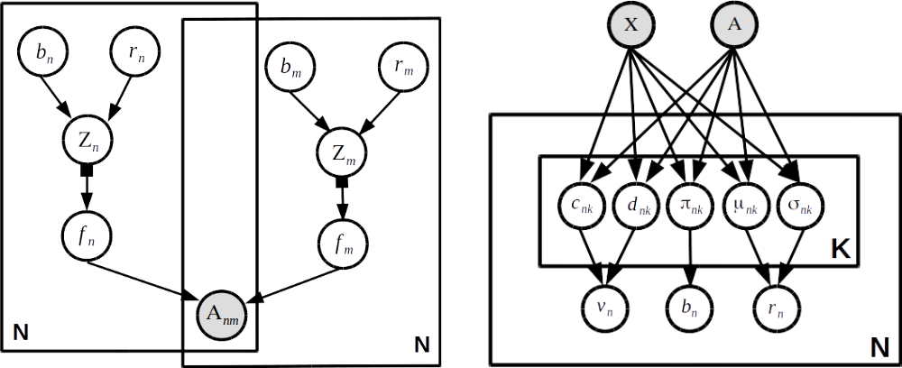
The decoder model (the left) is almost the same as the latent feature relational model:

$$p(A_{ij}| \cdot) = \sigma(f_{i}(z_{i})^{\top}f_{j}(z_{j}))$$ where $f_{i}$ is a neural network-like model for a vertex $i$ that maps a latent state $z_{i}$ to latent feature vectors.

I think the encoder part is more interesting:

• $q(v_{ik}) = \textsf{Beta}(c_{ik}, d_{ik})$

• $q(b_{ik}) = \textsf{Bernoulli}(c_{ik}, d_{ik})$

• $q(r_{i}) = \mathcal{N}(\mu_{i}, \textsf{diag}(\sigma_{i}^{2}))$

All these "variational" parameters are modelled by a neural network model mapping a full adjacency matrix $A$ and a feature matrix $X$. We can make sampling steps differentiable by approximate reparameterization tricks.