Variational inference of matrix factorization

fit.fqtl.factorize(
  y,
  k = 1,
  svd.init = TRUE,
  model = c("gaussian", "nb", "logit", "voom", "beta"),
  x.mean = NULL,
  c.mean = NULL,
  x.var = NULL,
  y.loc = NULL,
  y.loc2 = NULL,
  x.mean.loc = NULL,
  cis.dist = 1e+06,
  do.hyper = FALSE,
  tau = NULL,
  pi = NULL,
  tau.lb = -10,
  tau.ub = -4,
  pi.lb = -4,
  pi.ub = -1,
  tol = 1e-04,
  gammax = 1000,
  rate = 0.01,
  decay = 0,
  jitter = 0.1,
  nsample = 10,
  vbiter = 2000,
  verbose = TRUE,
  print.interv = 10,
  nthread = 1,
  rseed = NULL,
  options.mf = list(),
  options.reg = list()
)

Arguments

y: [n x m] response matrix
k: Rank of the factorization (default: 1)
svd.init: Initalize by SVD (default: TRUE)
model: choose an appropriate distribution for the generative model of y matrix from c('gaussian', 'nb', 'logit', 'voom', 'beta') (default: 'gaussian')
x.mean: [n x p] primary covariate matrix for mean change (can specify location)
c.mean: [n x q] secondary covariate matrix for mean change (dense)
x.var: [n x r] covariate marix for variance#'
y.loc: m x 1 genomic location of y variables
y.loc2: m x 1 genomic location of y variables (secondary)
x.mean.loc: p x 1 genomic location of x.mean variables
cis.dist: distance cutoff between x and y
do.hyper: Hyper parameter tuning (default: FALSE)
tau: Fixed value of tau
pi: Fixed value of pi
tau.lb: Lower-bound of tau (default: -10)
tau.ub: Upper-bound of tau (default: -4)
pi.lb: Lower-bound of pi (default: -4)
pi.ub: Upper-bound of pi (default: -1)
tol: Convergence criterion (default: 1e-4)
gammax: Maximum precision (default: 1000)
rate: Update rate (default: 1e-2)
decay: Update rate decay (default: 0)
jitter: SD of random jitter for mediation & factorization (default: 0.01)
nsample: Number of stochastic samples (default: 10)
vbiter: Number of variational Bayes iterations (default: 2000)
verbose: Verbosity (default: TRUE)
print.interv: Printing interval (default: 10)
nthread: Number of threads during calculation (default: 1)
rseed: Random seed
options.mf: A combined list of inference options for matrix factorization.
options.reg: A combined list of inference options for regression effects.

Value

a list of variational inference results

Details

Correct hidden confounders lurking in expression matrix using low-rank matrix factorization including genetic and other biological covariates. We estimate the following model:

mean $$\mathsf{E}[Y] = U V^{\top} + X \theta_{\mathsf{local}} + C \theta_{\mathsf{global}}$$

and variance $$\mathsf{V}[Y] = X_{\mathsf{var}} \theta_{\mathsf{var}}$$

We determined ranks by group-wise spike-slab prior imposed on the columns of U and V.

Author

Yongjin Park, ypp@stat.ubc.ca, ypp.ubc@gmail.com

Examples


 require(fqtl)
 require(Matrix)
 n <- 500
 m <- 100
 k <- 3
 p <- 200
 u <- matrix(rnorm(n * k), n, k)
 v <- matrix(rnorm(m * k), m, k)
 p.true <- 3
 theta.true <- matrix(sign(rnorm(1:p.true)), p.true, 1)
 X <- matrix(rnorm(n * p), n, p)
 y.resid <- X[,1:p.true] %*% theta.true
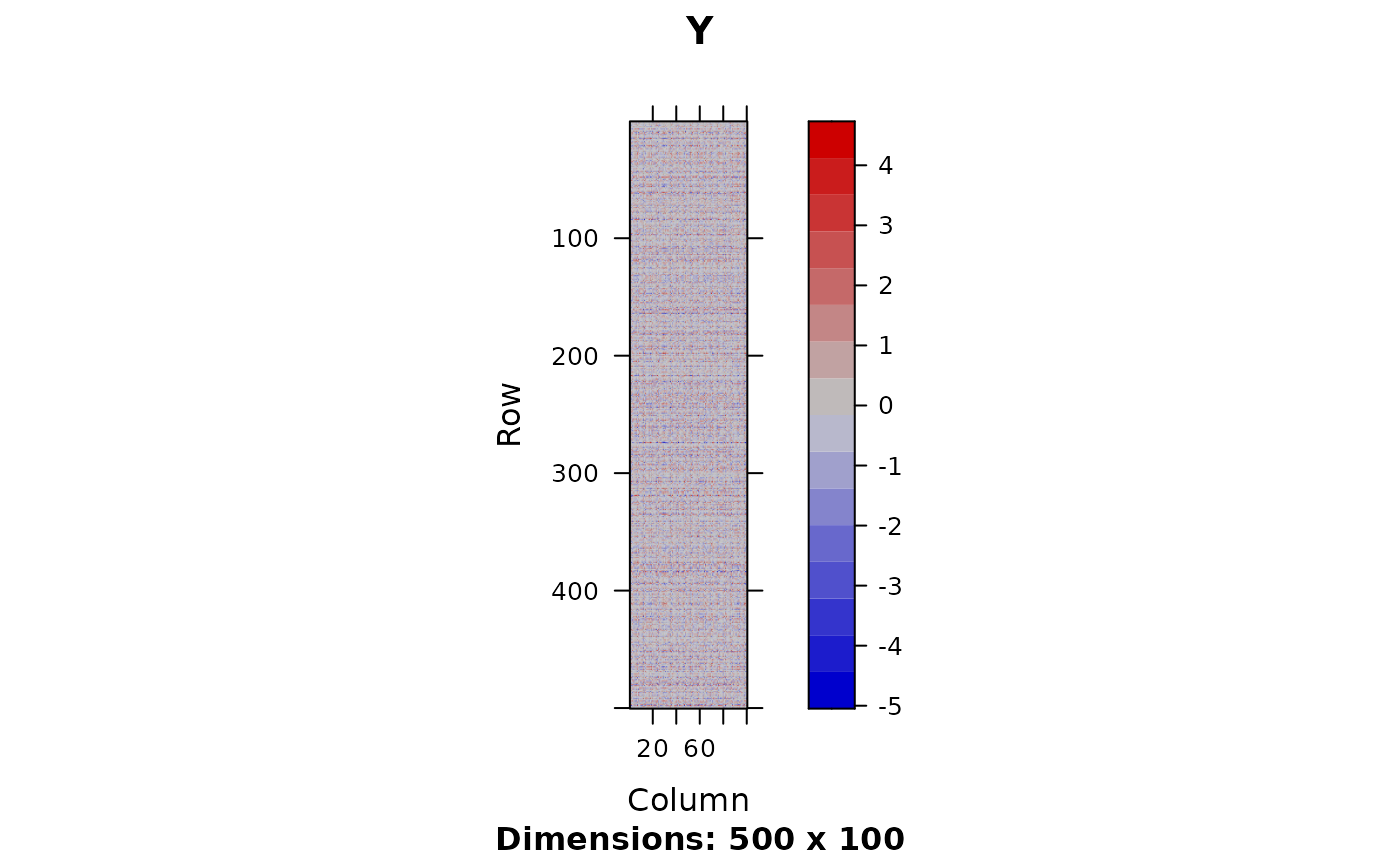
 y <- u %*% t(v) + 0.5 * matrix(rnorm(n * m), n, m)
 y[,1] <- y[,1] + y.resid
 y <- scale(y)
 x.v <- matrix(1, n, 1)
 xx <- as.matrix(cbind(X, 1))
 mf.opt <- list(tol=1e-8, rate=0.01, pi.ub=0, pi.lb=-2, svd.init = TRUE,
 jitter = 1e-1, vbiter = 1000, gammax=1e4, mf.pretrain = TRUE, k = 10)
 reg.opt <- list(pi.ub=-2, pi.lb=-4, gammax=1e4, vbiter = 1000)

## full t(xx) * y adjacency matrix
 mf.out <- fit.fqtl.factorize(y, x.mean = xx, x.var = x.v, options.mf = mf.opt)
 image(Matrix(y), main = 'Y')

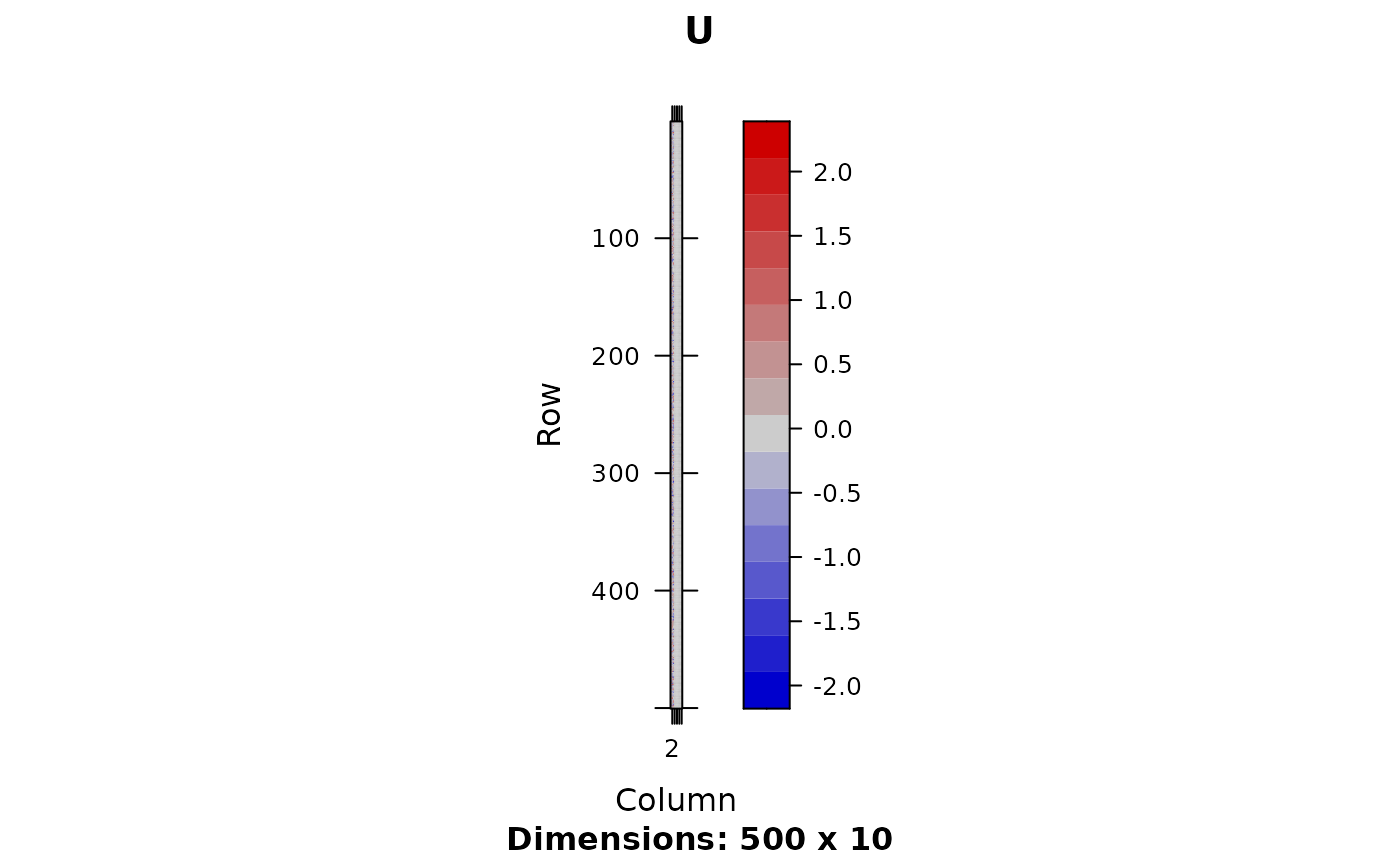
 image(Matrix(mf.out$U$theta), main = 'U')

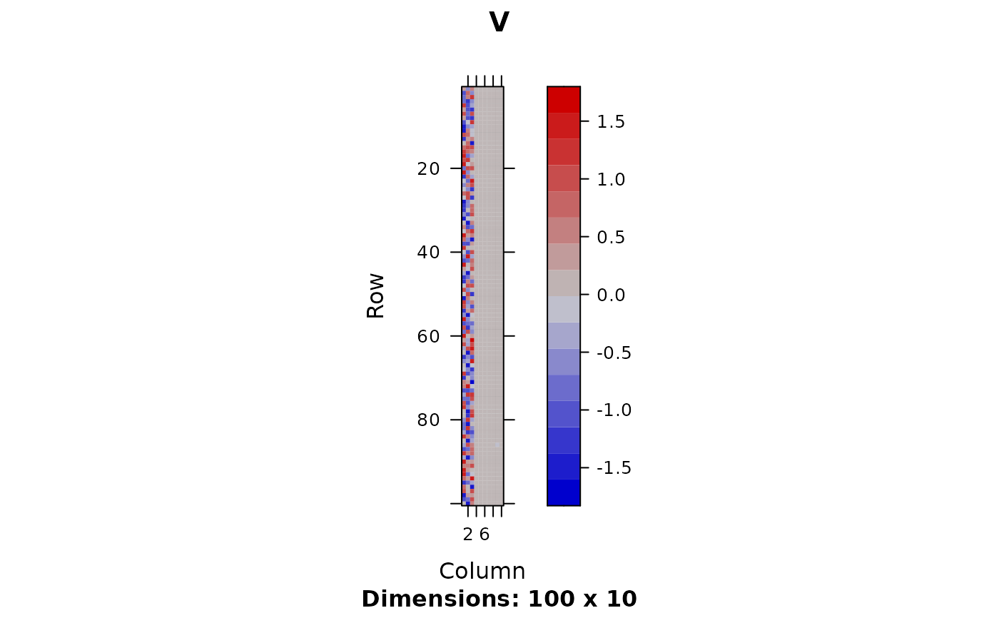
 image(Matrix(mf.out$V$theta), main = 'V')

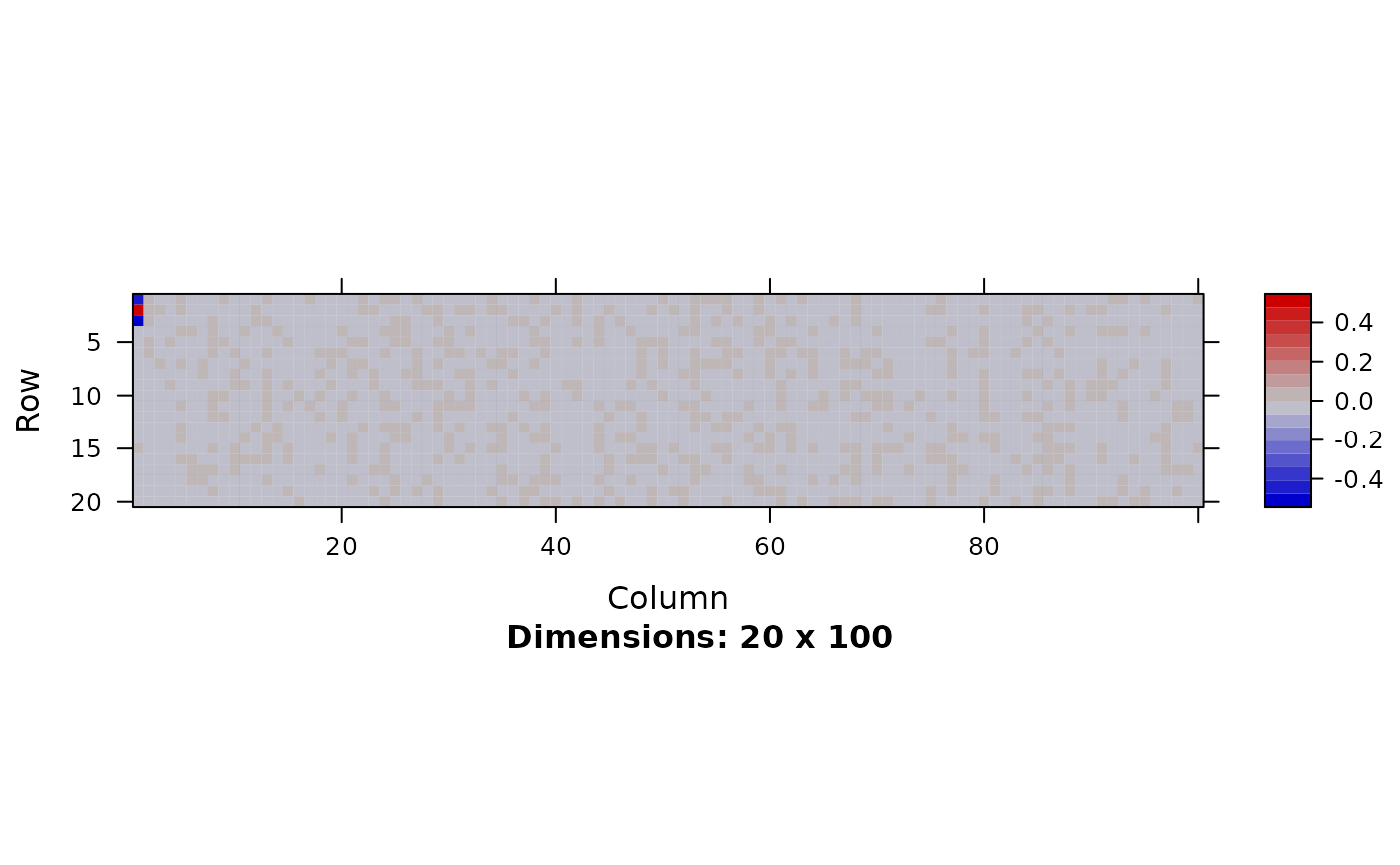
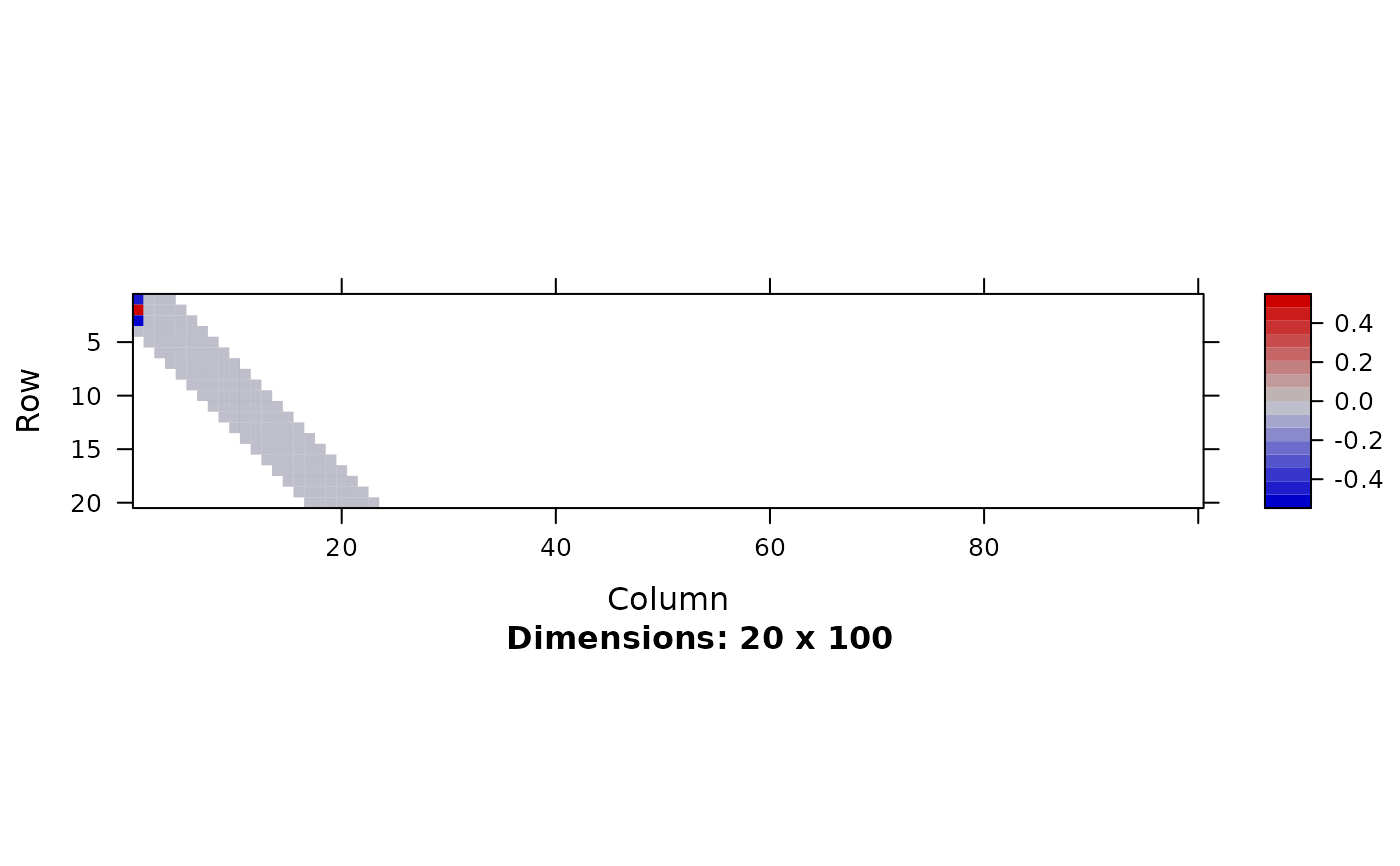
 image(Matrix(mf.out$mean$theta[1:20,]))


## sparse t(xx) * y adjacency matrix
 mf.out <- fit.fqtl.factorize(y, x.mean = xx, x.var = x.v, x.mean.loc = 1:(p+1),
                   y.loc = 1:m, cis.dist = 3,
                   options.mf = mf.opt,
                   options.reg = reg.opt)
 image(Matrix(mf.out$U$theta), main = 'U')

 image(Matrix(mf.out$V$theta), main = 'V')

 image(Matrix(mf.out$mean$theta[1:20,]))


## mixed, sparse and dense
 c.m <- matrix(1, n, 1)
 mf.out <- fit.fqtl.factorize(y, x.mean = xx, x.var = x.v, x.mean.loc = 1:(p+1),
                   y.loc = 1:m, cis.dist = 3, c.mean = c.m,
                   options.mf = mf.opt,
                   options.reg = reg.opt)
 image(Matrix(mf.out$U$theta), main = 'U')

 image(Matrix(mf.out$V$theta), main = 'V')