Variational deconvolution of matrix

fit.fqtl.deconv(
  y,
  weight.nk,
  svd.init = TRUE,
  model = c("gaussian", "nb", "logit", "voom", "beta"),
  x.mean = NULL,
  x.var = NULL,
  right.nn = FALSE,
  do.hyper = FALSE,
  tau = NULL,
  pi = NULL,
  tau.lb = -10,
  tau.ub = -4,
  pi.lb = -4,
  pi.ub = -1,
  tol = 1e-04,
  gammax = 1000,
  rate = 0.01,
  decay = 0,
  jitter = 0.1,
  nsample = 10,
  vbiter = 2000,
  verbose = TRUE,
  mu.min = 0.01,
  print.interv = 10,
  nthread = 1,
  rseed = NULL,
  options = list()
)

Arguments

y: [n x m] response matrix
weight.nk: (non-negative) weight matrix to help factors being mode interpretable
svd.init: Initalize by SVD (default: TRUE)
model: choose an appropriate distribution for the generative model of y matrix from c('gaussian', 'nb', 'logit', 'voom', 'beta') (default: 'gaussian')
x.mean: [n x p] covariate matrix for mean change (can specify location)
x.var: [n x r] covariate marix for variance#'
right.nn: non-negativity in factored effect (default: FALSE)
do.hyper: Hyper parameter tuning (default: FALSE)
tau: Fixed value of tau
pi: Fixed value of pi
tau.lb: Lower-bound of tau (default: -10)
tau.ub: Upper-bound of tau (default: -4)
pi.lb: Lower-bound of pi (default: -4)
pi.ub: Upper-bound of pi (default: -1)
tol: Convergence criterion (default: 1e-4)
gammax: Maximum precision (default: 1000)
rate: Update rate (default: 1e-2)
decay: Update rate decay (default: 0)
jitter: SD of random jitter for mediation & factorization (default: 0.01)
nsample: Number of stochastic samples (default: 10)
vbiter: Number of variational Bayes iterations (default: 2000)
verbose: Verbosity (default: TRUE)
mu.min: mininum non-negativity weight (default: 0.01)
print.interv: Printing interval (default: 10)
nthread: Number of threads during calculation (default: 1)
rseed: Random seed
options: A combined list of inference/optimization options

Examples


################################################################
## Simulate weighted matrix factorization (e.g., cell-type fraction)

n <- 600
p <- 1000
h2 <- 0.5

X <- matrix(rnorm(n * p), n, p)
Y <- matrix(rnorm(n * 1), n, 1) * sqrt(1 - h2)

## construct cell type specific genetic activities
K <- 3

causal <- NULL
eta <- matrix(nrow = n, ncol = K)

for(k in 1:K) {
  causal.k <- sample(p, 3)
  causal <- rbind(causal, data.frame(causal.k, k = k))
  eta[, k] <- eta.k <- X[, causal.k, drop = FALSE] %*% matrix(rnorm(3, 1) / sqrt(3), 3, 1)
}

## randomly sample cell type proportions from Dirichlet
rdir <- function(alpha) {
  ret <- sapply(alpha, rbeta, n = 1, shape2 = 1)
  ret <- ret / sum(ret)
  return(ret)
}

prop <- t(sapply(1:n, function(j) rdir(alpha = rep(1, K))))
eta.sum <- apply(eta * prop, 1, sum)
Y <- Y + eta.sum * sqrt(h2)

opt <- list(tol=1e-8, pi = -0, gammax=1e3, vbiter=10000, out.residual = FALSE,
do.hyper = FALSE, right.nn = TRUE)
out <- fit.fqtl.deconv(Y, prop, options = opt)

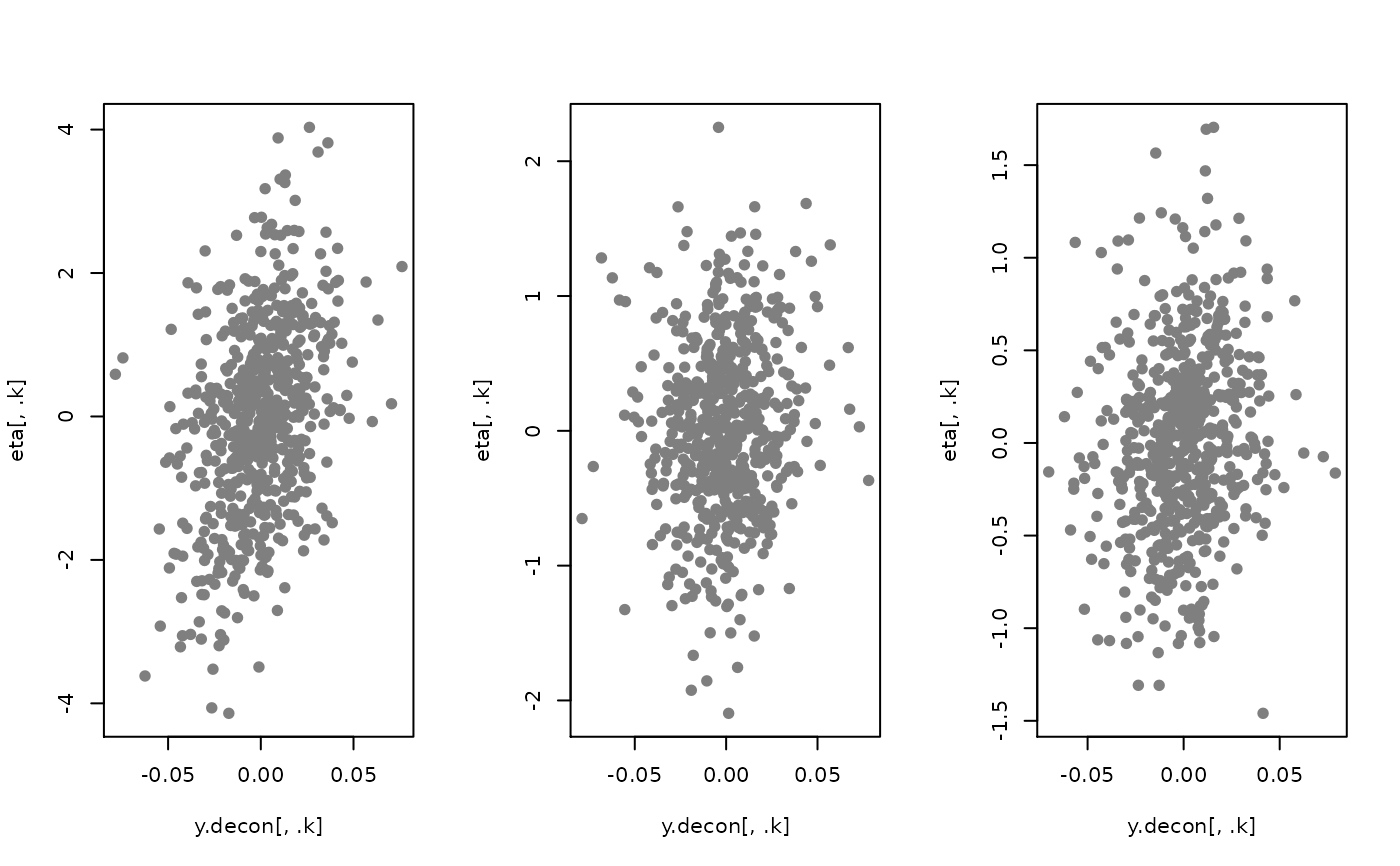
y.decon <- out$U$theta

par(mfrow = c(1, K))
for(.k in 1:K) {
  plot(y.decon[, .k], eta[, .k], pch = 19, col = 'gray50')
}